E step, Kalman filter

Inner working of the E step GLE_analysisEM.GLE_Estimator

Out:

/home/docs/checkouts/readthedocs.org/user_builds/gle-analysisem/checkouts/stable/examples/plot_e_step.py:17: FutureWarning: Passing a negative integer is deprecated in version 1.0 and will not be supported in future version. Instead, use None to not limit the column width.
  pd.set_option("display.max_colwidth", -1)
{'A': array([[ 0.02482259,  1.        ],
       [-1.        ,  3.07829865]]), 'C': array([[ 1.00000000e+00, -6.13716962e-17],
       [-6.13716962e-17,  1.00000000e+00]]), 'force': array([[-1.]]), 'µ_0': array([0.]), 'Σ_0': array([[1.]]), 'SST': array([[0.00024823, 0.        ],
       [0.        , 0.03078299]]), 'dt': 0.005, 'basis': {'basis_type': 'linear', 'transformer': None, 'dim_x': 1, 'nb_basis_elt': 1, 'mean': array([0.]), 'n_output_features': 1}}
/home/docs/checkouts/readthedocs.org/user_builds/gle-analysisem/checkouts/stable/GLE_analysisEM/_gle_estimator.py:103: RuntimeWarning: Mean of empty slice.
  hSdouble = 0.5 * np.log(detd[detd > 0.0]).mean()
/home/docs/checkouts/readthedocs.org/user_builds/gle-analysisem/conda/stable/lib/python3.9/site-packages/numpy/core/_methods.py:188: RuntimeWarning: invalid value encountered in double_scalars
  ret = ret.dtype.type(ret / rcount)
/home/docs/checkouts/readthedocs.org/user_builds/gle-analysisem/checkouts/stable/GLE_analysisEM/_gle_estimator.py:104: RuntimeWarning: Mean of empty slice.
  hSsimple = 0.5 * np.log(dets[dets > 0.0]).mean()
{'A': array([[ 0.02482259,  1.        ],
       [-1.        ,  3.07829865]]), 'C': array([[ 1.00000000e+00, -1.20384516e-16],
       [-1.33586700e-16,  1.00000000e+00]]), 'force': array([[-1.]]), 'µ_0': array([0.]), 'Σ_0': array([[1.]]), 'SST': array([[0.00024823, 0.        ],
       [0.        , 0.03078299]]), 'dt': 0.005, 'basis': {'basis_type': 'linear', 'transformer': None, 'dim_x': 1, 'nb_basis_elt': 1, 'mean': array([0.]), 'n_output_features': 1}}
Real datas
dxdx    [[0.0002958748244137596, 6.960496374804485e-05], [6.960496374804485e-05, 0.030957298275453626]]
xdx     [[-0.0001229072014013669, 0.005139064063362039], [-0.005201225244959364, -0.015548113886802328]]
xx      [[0.8180300869886296, 0.0026093126878508547], [0.0026093126878508547, 1.0277733045447912]]
bkx     [[0.002983451439285093, 0.01887440981152538]]
bkdx    [[-0.004069553029554174, -4.843456829261043e-05]]
bkbk    [[0.7999179036120212]]
µ_0     [0.0220131710573388]
Σ_0     [[0.0]]
hS      NaN
dtype: object
Estimated datas
dxdx    [[0.0002958748244137596, 7.758273846449614e-05], [7.758273846449614e-05, 0.031051442790759574]]
xdx     [[-0.0001229072014013669, 0.005118357590698583], [-0.005196967622153515, -0.015539721612355083]]
xx      [[0.8180300869886296, -0.0030046514929253534], [-0.0030046514929253534, 1.025317137685314]]
bkx     [[0.002983451439285093, 0.011651946687819088]]
bkdx    [[-0.004069553029554174, -2.683857017480784e-05]]
bkbk    [[0.7999179036120212]]
µ_0     [0.1284176896553403]
Σ_0     [[0.4137133453436859]]
hS     -0.342784
dtype: object
Diff
dxdx    [[0.0, 0.1146150258094974], [0.1146150258094974, 0.00304110890001652]]
xdx     [[0.0, -0.004029230305004091], [0.0008185807392162632, 0.000539761575477602]]
xx      [[0.0, -2.151510705066213], [-2.151510705066213, -0.0023897943725683683]]
bkx     [[0.0, -0.3826590179946184]]
bkdx    [[0.0, 0.4458798515005542]]
bkbk    [[0.0]]
µ_0     [4.833675181137892]
Σ_0     [[inf]]
hS      NaN
dtype: object
[[ 0.00015042  0.00501226]
 [-0.00620133  0.01513784]]
[[2.49404439e-04 3.29278927e-07]
 [3.29278927e-07 3.07844643e-02]] [[0.00024823 0.        ]
 [0.         0.03078299]]

import numpy as np
import pandas as pd
from matplotlib import pyplot as plt
from GLE_analysisEM import GLE_Estimator, GLE_BasisTransform, sufficient_stats, sufficient_stats_hidden

# Printing options
pd.set_option("display.max_rows", None)
pd.set_option("display.max_columns", None)
pd.set_option("display.width", None)
pd.set_option("display.max_colwidth", -1)

dim_x = 1
dim_h = 1
random_state = None
force = -np.identity(dim_x)
A = [[5, 1.0], [-1.0, 2.07]]
C = np.identity(dim_x + dim_h)  #
basis = GLE_BasisTransform(basis_type="linear")
generator = GLE_Estimator(verbose=1, dim_x=dim_x, dim_h=dim_h, basis=basis, C_init=C, force_init=force, init_params="random", random_state=random_state)
X, idx, Xh = generator.sample(n_samples=10000, n_trajs=10, x0=0.0, v0=0.0)
traj_list_h = np.split(Xh, idx)
time = np.split(X, idx)[0][:, 0]
for n, traj in enumerate(traj_list_h):
    traj_list_h[n] = traj_list_h[n][:-1, :]

print(generator.get_coefficients())

est = GLE_Estimator(init_params="user", dim_x=dim_x, dim_h=dim_h, basis=basis)
est.set_init_coeffs(generator.get_coefficients())
est.dt = time[1] - time[0]
est._check_initial_parameters()

Xproc, idx = est.model_class.preprocessingTraj(est.basis, X, idx_trajs=idx)
traj_list = np.split(Xproc, idx)
est.dim_coeffs_force = est.basis.nb_basis_elt_

datas = 0.0
for n, traj in enumerate(traj_list):
    datas_visible = sufficient_stats(traj, est.dim_x)
    zero_sig = np.zeros((len(traj), 2 * est.dim_h, 2 * est.dim_h))
    muh = np.hstack((np.roll(traj_list_h[n], -1, axis=0), traj_list_h[n]))
    datas += sufficient_stats_hidden(muh, zero_sig, traj, datas_visible, est.dim_x, est.dim_h, est.dim_coeffs_force) / len(traj_list)

est._initialize_parameters(None)
print(est.get_coefficients())
print("Real datas")
print(datas)
new_stat = 0.0
noise_corr = 0.0
for n, traj in enumerate(traj_list):
    datas_visible = sufficient_stats(traj, est.dim_x)
    muh, Sigh = est._e_step(traj)  # Compute hidden variable distribution
    new_stat += sufficient_stats_hidden(muh, Sigh, traj, datas_visible, est.dim_x, est.dim_h, est.dim_coeffs_force) / len(traj_list)
print("Estimated datas")
print(new_stat)
print("Diff")
print((new_stat - datas) / np.abs(datas))


Pf = np.zeros((dim_x + dim_h, dim_x))
Pf[:dim_x, :dim_x] = 5e-3 * np.identity(dim_x)
YX = new_stat["xdx"].T - np.matmul(Pf, np.matmul(force, new_stat["bkx"]))
XX = new_stat["xx"]
A = -np.matmul(YX, np.linalg.inv(XX))


Pf = np.zeros((dim_x + dim_h, dim_x))
Pf[:dim_x, :dim_x] = 5e-3 * np.identity(dim_x)

# A = generator.friction_coeffs
print(A)
bkbk = np.matmul(Pf, np.matmul(np.matmul(force, np.matmul(new_stat["bkbk"], force.T)), Pf.T))
bkdx = np.matmul(Pf, np.matmul(force, new_stat["bkdx"]))
bkx = np.matmul(Pf, np.matmul(force, new_stat["bkx"]))

residuals = new_stat["dxdx"] + np.matmul(A, new_stat["xdx"]) + np.matmul(A, new_stat["xdx"]).T - bkdx.T - bkdx
residuals += np.matmul(A, np.matmul(new_stat["xx"], A.T)) - np.matmul(A, bkx.T) - np.matmul(A, bkx.T).T + bkbk
print(residuals, generator.diffusion_coeffs)
# SST = 0.5 * (residuals + residuals.T)

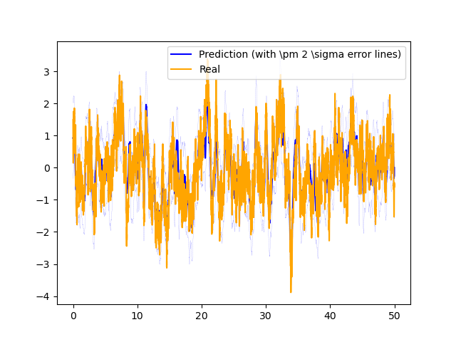
fig, axs = plt.subplots(1, dim_h)
# plt.show()
for k in range(dim_h):
    axs.plot(time[:-1], muh[:, k], label="Prediction (with \\pm 2 \\sigma error lines)", color="blue")
    axs.plot(time[:-1], muh[:, k] + 2 * np.sqrt(Sigh[:, k, k]), "--", color="blue", linewidth=0.1)
    axs.plot(time[:-1], muh[:, k] - 2 * np.sqrt(Sigh[:, k, k]), "--", color="blue", linewidth=0.1)
    axs.plot(time[:-1], traj_list_h[n][:, k], label="Real", color="orange")
    axs.legend(loc="upper right")
plt.show()